
| 일 | 월 | 화 | 수 | 목 | 금 | 토 |
|---|---|---|---|---|---|---|
| 1 | 2 | 3 | 4 | 5 | ||
| 6 | 7 | 8 | 9 | 10 | 11 | 12 |
| 13 | 14 | 15 | 16 | 17 | 18 | 19 |
| 20 | 21 | 22 | 23 | 24 | 25 | 26 |
| 27 | 28 | 29 | 30 |
- 이것이 코딩테스트다
- pandas
- sklearn
- scikit learn
- 태블로
- 데이터 분석
- 자격증
- 이코테
- 시각화
- Google ML Bootcamp
- 파이썬
- 코딩테스트
- 통계
- ML
- ADsP
- Python
- r
- pytorch
- matplotlib
- 딥러닝
- tableau
- IRIS
- 데이터 전처리
- 머신러닝
- SQL
- Deep Learning Specialization
- 데이터분석
- 데이터분석준전문가
- 회귀분석
- SQLD
- Today
- Total
함께하는 데이터 분석
[EDA] FA with R 본문
안녕하세요!
오늘은 Factor Analysis의 약자인 FA에 대해 알아보겠습니다.
파일은 저번이랑 똑같은
이 파일입니다. 만약 파일 정보가 필요하시다면
2022.02.06 - [분류 전체보기] - [EDA] PCA with R
[EDA] PCA with R
오늘은 Principal Component Analysis 일명 PCA에 대해 간단한 예제를 R을 통해 알아보는 시간을 갖겠습니다! 그러기에 앞서 필요한 파일을 첨부하겠습니다. 위 데이터는 주식에 관한 10개 회사의 값입니
tnqkrdmssjan.tistory.com
여기서 확인해주세요!
그럼 시작하겠습니다.
### perfrom factor analysis with 3 factors but without any rotation
kval<-3 #앞서 PCA와 hclust의 결과를 토대로 3개의 factor로 해보기

stock.FA<-factanal(scale(stocks), kval, rotation="none")
## varimax rotation (orthogonal rotation)
stock.FAr1<-factanal(scale(stocks), kval, rotation="varimax")
## promax rotation (oblique rotation)
stock.FAr2<-factanal(scale(stocks), kval, rotation="promax")
여기서는 앞서 PCA와 hclust의 결과를 토대로 3개의 factor로 분석했지만
만약 결과를 알 수 없을 땐 2, 3, 4, 등등 여러 가지 경우를 돌려보고
유의미한 factor 개수를 찾아야 합니다.
FA를 할 때 rotation 종류에 따라 3가지 방법 no rotation, varimax, promax이 있습니다.
그중 가장 유의미하다고 생각되는 것을 골라서 사용하면 됩니다.
## with no rotation
with(stock.FA, plot(loadings[,1], loadings[,2], xlim=c(-1, 1), ylim=c(-1,1),
                    main="Stocks (No rotation)", xlab="Factor 1", ylab="Factor 2"))
with(stock.FA, text(loadings[,1], loadings[,2],labels=1:10, pos=4))
abline(v=0); abline(h=0)
with(stock.FA, plot(loadings[,1], loadings[,3], xlim=c(-1, 1), ylim=c(-1,1),
                    main="Stocks (No rotation)", xlab="Factor 1", ylab="Factor 3"))
with(stock.FA, text(loadings[,1], loadings[,3],labels=1:10, pos=4))
abline(v=0); abline(h=0)
위의 경우는 rotation을 하지 않은 경우인데 그래프를 보면
구별하기 쉽지 않은 것을 알 수 있습니다.
stock.FA$loadings
>>> Loadings:
           Factor1 Factor2 Factor3
    comp1   0.889   0.237  -0.235
    comp2   0.713   0.386
    comp3   0.335   0.278
    comp4   0.309   0.111  -0.191
    comp5   0.628  -0.664   0.148
    comp6   0.473  -0.638
    comp7   0.113  -0.542
    comp8   0.640   0.167   0.496
    comp9   0.236   0.529   0.577
    comp10  0.110   0.168   0.552

                   Factor1 Factor2 Factor3
    SS loadings      2.613   1.773   0.999
    Proportion Var   0.261   0.177   0.100
    Cumulative Var   0.261   0.439   0.539
## with varimax
with(stock.FAr1, plot(loadings[,1], loadings[,2], xlim=c(-1, 1), ylim=c(-1,1),
                      main="Stocks (Varimax)", xlab="Factor 1", ylab="Factor 2"))
with(stock.FAr1, text(loadings[,1], loadings[,2],labels=1:10, pos=4))
abline(v=0); abline(h=0)

with(stock.FAr1, plot(loadings[,1], loadings[,3], xlim=c(-1, 1), ylim=c(-1,1),
                      main="Stocks (Varimax)", xlab="Factor 1", ylab="Factor 3"))
with(stock.FAr1, text(loadings[,1], loadings[,3],labels=1:10, pos=4))
abline(v=0); abline(h=0)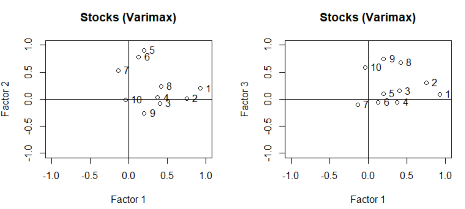
위의 경우는 varimax rotation을 사용한 경우인데 첫 번째 그래프를 보면
comp5, 6, 7이 뭉쳐있고 Factor2가 큰 것을 확인할 수 있습니다.
stock.FAr1$loadings
>>> Loadings:
           Factor1 Factor2 Factor3
    comp1   0.924   0.197
    comp2   0.751           0.305
    comp3   0.401           0.151
    comp4   0.374
    comp5   0.195   0.899   0.103
    comp6   0.126   0.782
    comp7  -0.140   0.526  -0.102
    comp8   0.418   0.238   0.673
    comp9   0.200  -0.260   0.749
    comp10                  0.586

                   Factor1 Factor2 Factor3
    SS loadings      2.009   1.869   1.508
    Proportion Var   0.201   0.187   0.151
    Cumulative Var   0.201   0.388   0.539
comp1, 2, 3, 4는 Factor1
comp5, 6, 7은 Factor2
comp8, 9, 10은 Factor3의 값이 큰 것을 확인할 수 있습니다!
즉, 각각의 Factor가 해당하는 회사에 유의미하게 작용한다는 것을 알 수 있죠.
## with promax
with(stock.FAr2, plot(loadings[,1], loadings[,2], xlim=c(-1, 1), ylim=c(-1,1),
                      main="Stocks (Promax)", xlab="Factor 1", ylab="Factor 2"))
with(stock.FAr2, text(loadings[,1], loadings[,2],labels=1:10, pos=4))
abline(v=0); abline(h=0)

with(stock.FAr2, plot(loadings[,1], loadings[,3], xlim=c(-1, 1), ylim=c(-1,1),
                      main="Stocks (Promax)", xlab="Factor 1", ylab="Factor 3"))
with(stock.FAr2, text(loadings[,1], loadings[,3],labels=1:10, pos=4))
abline(v=0); abline(h=0)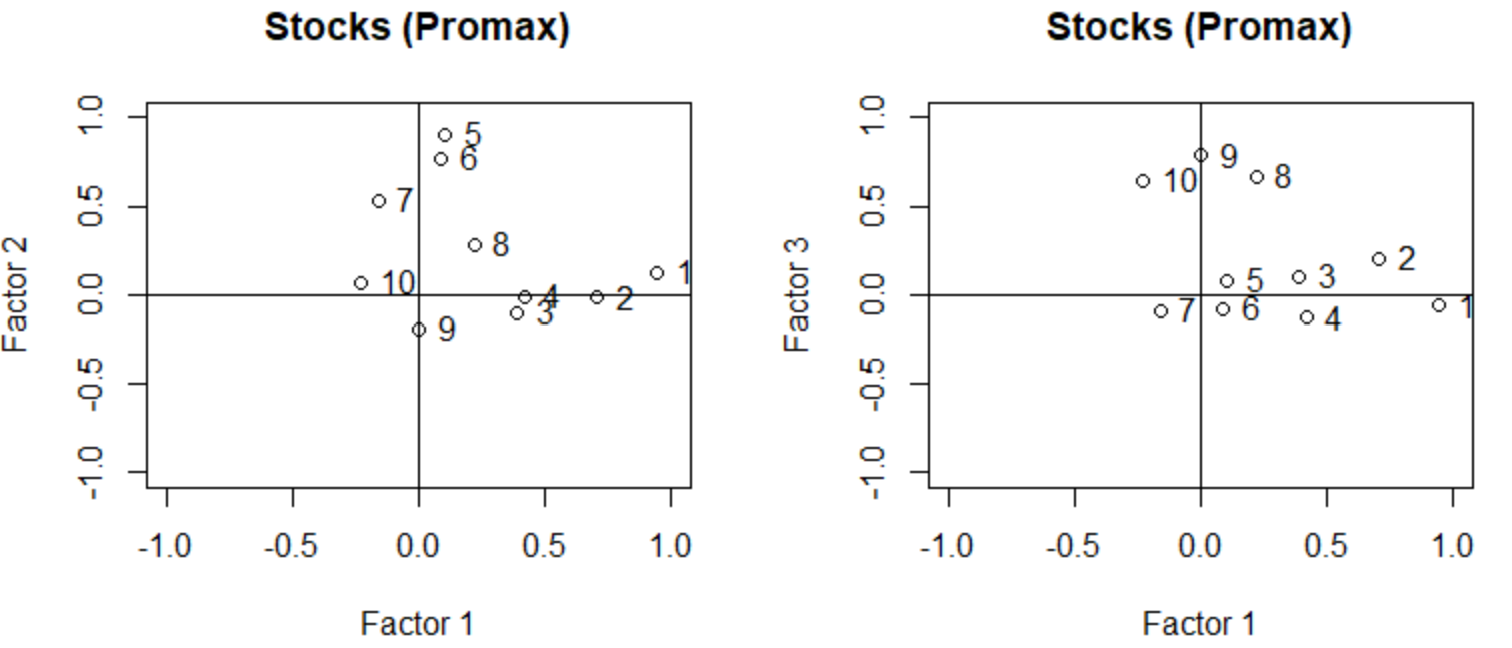
마지막으로 promax rotation입니다.
첫 번째 그래프에서 comp5, 6, 7이 Factor2에 영향을 받고
두 번째 그래프에서 comp8, 9, 10이 Factor3에 영향을 받는다는 것을
쉽게 볼 수 있죠!
stock.FAr2$loadings
>>> Loadings:
           Factor1 Factor2 Factor3
    comp1   0.945   0.121
    comp2   0.706           0.206
    comp3   0.388
    comp4   0.416          -0.130
    comp5   0.102   0.902
    comp6           0.771
    comp7  -0.162   0.532
    comp8   0.217   0.284   0.664
    comp9          -0.188   0.785
    comp10 -0.229           0.648

                   Factor1 Factor2 Factor3
    SS loadings      1.860   1.836   1.569
    Proportion Var   0.186   0.184   0.157
    Cumulative Var   0.186   0.370   0.527
이 결과를 보더라도 위의 no rotation, varimax rotation보다 더 쉽게
결과를 도출할 수 있죠.
이처럼 3가지 rotation 중 본인이 분석할 때 더 유의미하다고 생각되는 것을
사용하면 됩니다.
감사합니다!

'통계학과 수업 기록 > EDA' 카테고리의 다른 글
| [EDA] PCA with R (0) | 2022.02.06 |
|---|---|
| [EDA] SVD with R (0) | 2022.02.05 |
| [EDA] K-Means Clustering with R (0) | 2022.02.02 |
| [EDA] Hierarchical Clustering with R (0) | 2022.02.02 |


