| 일 | 월 | 화 | 수 | 목 | 금 | 토 |
|---|---|---|---|---|---|---|
| 1 | 2 | 3 | 4 | 5 | 6 | 7 |
| 8 | 9 | 10 | 11 | 12 | 13 | 14 |
| 15 | 16 | 17 | 18 | 19 | 20 | 21 |
| 22 | 23 | 24 | 25 | 26 | 27 | 28 |
| 29 | 30 |
- 시각화
- Deep Learning Specialization
- IRIS
- 딥러닝
- ML
- 이것이 코딩테스트다
- scikit learn
- sklearn
- 자격증
- 데이터 분석
- 태블로
- 코딩테스트
- 회귀분석
- ADsP
- 데이터 전처리
- r
- pandas
- SQLD
- tableau
- matplotlib
- 데이터분석준전문가
- 데이터분석
- 머신러닝
- 파이썬
- 통계
- pytorch
- Google ML Bootcamp
- Python
- SQL
- 이코테
- Today
- Total
함께하는 데이터 분석
[Find-A][Scikit Learn] 앙상블 학습 본문
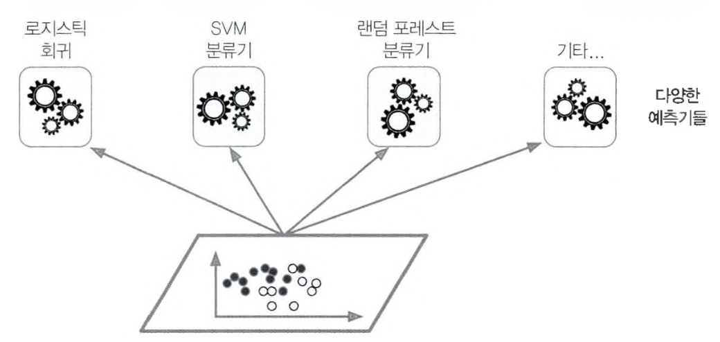
앙상블 학습
- 가장 좋은 모델 하나보다 비슷한 일련의 예측기로부터 예측을 수집하여 더 좋은 예측을 얻는 것
투표 기반 분류기
정확도가 80% 정도 되는 분류기를 여러 개 훈련시켰다고 가정
더 좋은 분류기를 만드는 매우 간단한 방법은 각 분류기의 예측을 모아 가장 많이 선택된 클래스를 예측
이렇게 다수결의 투표 즉, 통계적 최빈값으로 정해지는 분류기를 직접 투표(hard voting)이라 함
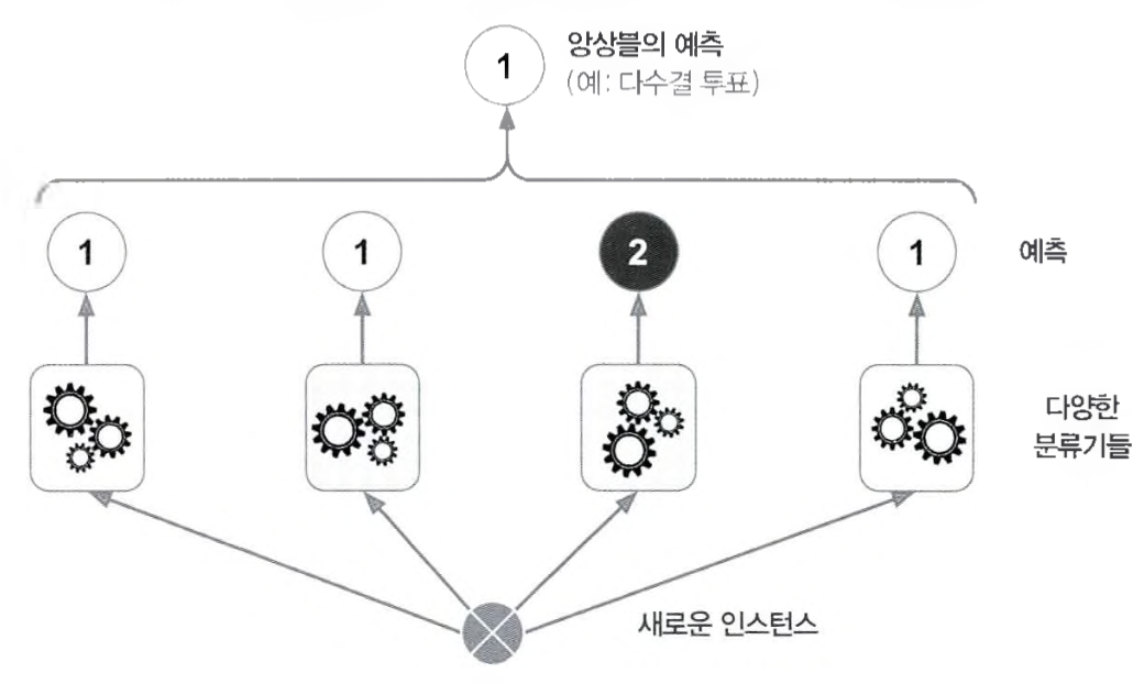
이 다수결 투표 분류기가 앙상블에 포함된 개별 분류기 중 가장 뛰어난 것보다 정확도가 높은 경우가 많음
각 분류기가 약한 학습기(weak learner)일지라도 많고 다양하면 앙상블은 강한 학습기(strong learner)가 될 수 있음
큰 수의 법칙
import numpy as np
import pandas as pd
import seaborn as sns
import matplotlib.pyplot as plt
import sklearn
import warnings
warnings.filterwarnings('ignore')
heads_proba = 0.51
coin_tosses = (np.random.rand(10000, 10) < heads_proba).astype(np.int32)
cumulative_heads_ratio = np.cumsum(coin_tosses, axis=0) / np.arange(1, 10001).reshape(-1, 1)plt.rc('font', family='AppleGothic')
plt.rc('font', size=12)
plt.rc('axes', unicode_minus=False)
plt.figure(figsize=(8, 4))
plt.plot(cumulative_heads_ratio)
plt.plot([0, 10000], [0.51, 0.51], "k--", linewidth=2, label="51%")
plt.plot([0, 10000], [0.5, 0.5], "k-", label="50%")
plt.xlabel("동전을 던진 횟수")
plt.ylabel("앞면이 나온 비율")
plt.legend(loc="lower right")
plt.axis([0, 10000, 0.42, 0.58])
plt.show()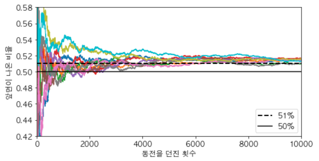
동전을 던졌을 때 앞면이 51%, 뒷면이 49%가 나오는 동전이 있다고 가정
1000번 던진다면 대략 510번은 앞면, 490번은 뒷면이 나올 것이므로 다수는 앞면
이항 분포를 이용하여 1000의 과반 직전인 499까지의 확률을 더하여 전체 확률 1에서 빼면
1000번 던져 앞면이 절반 이상 나올 확률이 됨
from scipy.stats import binom

1-binom.cdf(499, 1000, 0.51)

>>> 0.7467502275563251
이와 비슷하게 51% 정확도를 가진 1000개의 분류기로 앙상블 모델을 구축하고
가장 많은 클래스를 예측으로 삼는다면 75%의 정확도를 기대할 수 있음
하지만 이는 동전과 마찬가지로 독립이어야 하고 오차에 상관관계가 없어야 가능
따라서 앙상블 방법은 예측기가 가능한 한 서로 독립일 때 즉, 각기 다른 알고리즘으로 학습시킬 때 정확도가 좋음
투표 기반 분류기 훈련
from sklearn.model_selection import train_test_split
from sklearn.datasets import make_moons

X, y = make_moons(n_samples=500, noise=0.3, random_state=42)
X_train, X_test, y_train, y_test = train_test_split(X, y, random_state=42)
사이킷런의 moons 데이터셋을 훈련 세트와 테스트 세트로 분리
from sklearn.ensemble import RandomForestClassifier
from sklearn.ensemble import VotingClassifier
from sklearn.linear_model import LogisticRegression
from sklearn.svm import SVC

log_clf = LogisticRegression(solver='liblinear', random_state=42)
rnd_clf = RandomForestClassifier(n_estimators=10, random_state=42)
svm_clf = SVC(gamma='auto', random_state=42)

voting_clf = VotingClassifier(
    estimators=[('lr', log_clf), ('rf', rnd_clf), ('svc', svm_clf)],
    voting='hard')
voting_clf.fit(X_train, y_train)
개별 분류기로 로지스틱 회귀, 랜덤 포레스트, SVM을 선택하고 학습시킴
추가로 투표 기반 분류기로도 학습(hard voting)
from sklearn.metrics import accuracy_score

for clf in (log_clf, rnd_clf, svm_clf, voting_clf):
    clf.fit(X_train, y_train)
    y_pred = clf.predict(X_test)
    print(clf.__class__.__name__, accuracy_score(y_test, y_pred))

>>> LogisticRegression 0.864
    RandomForestClassifier 0.872
    SVC 0.888
    VotingClassifier 0.896
다른 개별 분류기보다 투표 기반 분류기가 성능이 좋음
여기서 통계적 최빈값을 활용하는 hard voting이 아니라 개별 분류기의 예측의 평균을 활용하는 간접투표(soft voting)가 있음
log_clf = LogisticRegression(solver='liblinear', random_state=42)
rnd_clf = RandomForestClassifier(n_estimators=10, random_state=42)
svm_clf = SVC(gamma='auto', probability=True, random_state=42)

voting_clf = VotingClassifier(
    estimators=[('lr', log_clf), ('rf', rnd_clf), ('svc', svm_clf)],
    voting='soft')
voting_clf.fit(X_train, y_train)
voting='hard'를 voting='soft'로 바꾸면 사용 가능
from sklearn.metrics import accuracy_score

for clf in (log_clf, rnd_clf, svm_clf, voting_clf):
    clf.fit(X_train, y_train)
    y_pred = clf.predict(X_test)
    print(clf.__class__.__name__, accuracy_score(y_test, y_pred))

>>> LogisticRegression 0.864
    RandomForestClassifier 0.872
    SVC 0.888
    VotingClassifier 0.912
soft voting은 확률이 높은 투표에 비중을 더 두기 때문에 hard voting보다 성능이 좋음
배깅과 페이스팅
다양한 분류기를 만드는 한 가지 방법은 각기 다른 훈련 알고리즘을 사용하는 것
또 다른 방법은 같은 알고리즘을 사용하지만 훈련 세트의 표본을 무작위로 구성하여 분류기를 각기 다르게 학습시키는 것
중복을 허용하여 샘플링하는 방식을 배깅(bagging), 중복을 허용하지 않고 샘플링하는 방식을 페이스팅(pasting)이라 함
하지만 배깅만이 한 예측기를 위해 같은 훈련 샘플을 여러 번 샘플링할 수 있음

모든 예측기가 훈련을 마치면 앙상블은 모든 예측기의 예측을 모아서 새로운 샘플에 대한 예측을 만듦
수집 함수는 분류일 때는 통계적 최빈값, 회귀일 때는 평균을 계산
개별 예측기는 원본 훈련 세트로 훈련시킨 것보다 훨씬 크게 편향되어 있지만 수집 함수를 통과하면 편향과 분산이 모두 감소
따라서 일반적으로 원본 데이터셋으로 하나의 예측기를 훈련시킬 때와 비교하면 편향은 비슷하지만 분산은 감소
배깅과 페이스팅 훈련
from sklearn.ensemble import BaggingClassifier
from sklearn.tree import DecisionTreeClassifier

bag_clf = BaggingClassifier(
    DecisionTreeClassifier(random_state=42), n_estimators=500,
    max_samples=100, bootstrap=True, n_jobs=-1, random_state=42)
bag_clf.fit(X_train, y_train)
y_pred = bag_clf.predict(X_test)
의사결정 나무 분류기 500개의 앙상블을 훈련시키는 코드
각 분류기는 훈련 세트에서 중복을 허용하여 무작위로 100개의 샘플로 훈련
bootstrap을 False로 지정하면 비 복원으로 페이스팅이 됨
n_jobs 매개변수는 훈련과 예측에 사용할 CPU 코어 수를 지정하고 -1은 가용한 모든 코어를 사용
from sklearn.metrics import accuracy_score
print(accuracy_score(y_test, y_pred))

>>> 0.904
정확도가 90.4%가 나오는 것을 확인 가능
tree_clf = DecisionTreeClassifier(random_state=42)
tree_clf.fit(X_train, y_train)
y_pred_tree = tree_clf.predict(X_test)
단일 의사결정 나무 분류기를 사용하는 코드
from sklearn.metrics import accuracy_score
print(accuracy_score(y_test, y_pred_tree))

>>> 0.856
정확도가 85.6%로 배깅을 사용한 것보다 성능이 떨어짐
결정 경계
from matplotlib.colors import ListedColormap

def plot_decision_boundary(clf, X, y, axes=[-1.5, 2.5, -1, 1.5], alpha=0.5, contour=True):
    x1s = np.linspace(axes[0], axes[1], 100)
    x2s = np.linspace(axes[2], axes[3], 100)
    x1, x2 = np.meshgrid(x1s, x2s)
    X_new = np.c_[x1.ravel(), x2.ravel()]
    y_pred = clf.predict(X_new).reshape(x1.shape)
    custom_cmap = ListedColormap(['#fafab0','#9898ff','#a0faa0'])
    plt.contourf(x1, x2, y_pred, alpha=0.3, cmap=custom_cmap)
    if contour:
        custom_cmap2 = ListedColormap(['#7d7d58','#4c4c7f','#507d50'])
        plt.contour(x1, x2, y_pred, cmap=custom_cmap2, alpha=0.8)
    plt.plot(X[:, 0][y==0], X[:, 1][y==0], "yo", alpha=alpha)
    plt.plot(X[:, 0][y==1], X[:, 1][y==1], "bs", alpha=alpha)
    plt.axis(axes)
    plt.xlabel(r"$x_1$", fontsize=12)
    plt.ylabel(r"$x_2$", fontsize=12, rotation=0)

plt.figure(figsize=(11,4))
plt.subplot(121)
plot_decision_boundary(tree_clf, X, y)
plt.title("Decision Tree", fontsize=14)
plt.subplot(122)
plot_decision_boundary(bag_clf, X, y)
plt.title("배깅을 사용한 Decision Tree", fontsize=14)
plt.show()
왼쪽은 단일 Decision Tree의 결정 경계이고 오른쪽은 500개의 Decision Tree를 사용한 배깅 앙상블의 결정 경계
배깅 앙상블의 예측이 Decision Tree 하나의 예측보다 일반화가 잘 되는 것 확인 가능
https://www.hanbit.co.kr/store/books/look.php?p_code=B9267655530
핸즈온 머신러닝
최근의 눈부신 혁신들로 딥러닝은 머신러닝 분야 전체를 뒤흔들고 있습니다. 이제 이 기술을 거의 모르는 프로그래머도 데이터로부터 학습하는 프로그램을 어렵지 않게 작성할 수 있습니다. 이
www.hanbit.co.kr
'학회 세션 > 파인드 알파' 카테고리의 다른 글
| [Find-A] LSTM, GRU, 임베딩 (1) | 2022.09.21 |
|---|---|
| [Find-A] 인공 신경망 (0) | 2022.09.12 |
| [Find-A][Scikit Learn] Decision Tree (0) | 2022.08.24 |
| [Find-A] [Scikit Learn] 소프트맥스 회귀 (0) | 2022.08.20 |
| [Find-A] [Scikit Learn] 로지스틱 회귀 (0) | 2022.08.19 |